In this blog, we used toy models to reconstruct 3D chromatin structure. This problem is posed as an optimization problem. The input is 3D distance derived from Hi-C and FISH data, and the output is the relative coordinates in 3D space.

We consider the DNA sequence as a loop of beads (several consecutive sequences are one bead).

Here are the experimental procedures for Hi-C. Hi-C will return the interaction frequency of pairwise beads. Intuitively, when the distance of two beads is close, their interaction frequency is large. If the relationship between spatial distance and interaction frequency is strictly positive correlated. We could just use the interaction frequency to reconstruct the structure. However, Hi-C data has much noise when the interaction frequency is too large or small. Since we don't know the threshold, we could integrate FISH data (the determined distance of two beads) and pose the problem as a curve fitting problem.

To pose it as an optimization problem, we want to make the pairwise distance from estimated coordinates as close as the real distance. Thus, the objective function is defined using mean-squared error between actual distances and calculated distances, and initial coordinates for all the positions are randomly initialized within a ball with radius 1.0.the objective function here. More precisely, $$F_n = \sum_{i < j}\frac{(||P_i - P_j|| - D_{ij})^2}{D_{ij}^2}.$$ We could use gradient descent to solve this problem. The derivatives used for updating parameters are $$\frac{\partial F_n}{\partial x_i}=\ sum_j \frac{2(||P_i - P_j|| - D_{ij})^2}{D_{ij}^2} \frac{x_i-x_j}{\sqrt{(x_i-x_j)^2+(y_i-y_j)^2 +(z_i-z_j)^2}}$$ $$\frac{\partial F_n}{\partial y_i}=\ sum_j \frac{2(||P_i - P_j|| - D_{ij})^2}{D_{ij}^2} \frac{y_i-y_j}{\sqrt{(x_i-x_j)^2+(y_i-y_j)^2 +(z_i-z_j)^2}}$$ $$\frac{\partial F_n}{\partial z_i}=\ sum_j \frac{2(||P_i - P_j|| - D_{ij})^2}{D_{ij}^2} \frac{z_i-z_j}{\sqrt{(x_i-x_j)^2+(y_i-y_j)^2 +(z_i-z_j)^2}}$$ The coordinate update process for node i is $$x_i=x _i - lr * \frac{\partial F_n}{\partial x_i}$$ $$y_i=y _i - lr * \frac{\partial F_n}{\partial y_i}$$ $$z_i=z _i - lr * \frac{\partial F_n}{\partial z_i}$$

Given FISH data is hard to get, model 2 only used Hi-C data. More precisely, we used the following equation for normalization: $$F_{ij}= C_{ij} \frac{\sum_{k=1}^{n-1} \sum_{l=k+1}^n C_{kl}}{\sum_{k=1}^n C_{ik} \sum_{k=1}^n C_{kj}}$$ where $C_ij$ are the contract frequency from Hi-C.

The goal of optimization using Lorentzian objective function is to make the distances between region pairs in contact less than dc (contact distance threshold) and the distances between non- contact regions at least dc[7]. The weight parameters are used with the objective function below to guide the reconstruction of chromosomal structures: $$F_n = \sum_{contacts, |i - j| \ne 1} (W_1 tanh(d_c^2-d_{ij}^2) \frac{F_{ij}}{totalIF} + W_2\frac{tanh(d_{ij}^2 - d_{min}^2)}{totalIF}) \\ + \sum_{non-contacts, |i - j| \ne 1} (W_3 \frac{tanh(d_{max}^2-d_{ij}^2)}{totalIF} + W_4\frac{tanh(d_{ij}^2 - d_{min}^2)}{totalIF}) \\ + \sum_{|i - j| = 1} (W_1 tanh(da_{max}^2-d_{ij}^2) \frac{IF_{max}}{totalIF} + W_2\frac{tanh(d_{ij}^2 - d_{min}^2)}{totalIF})$$

Here dmin, dmax and damax are some parameters we chose based on prior knowledge[7]. To specify, dmin is the minimum distance between two regions, and dmax is the maximum distance between two regions. damax is the maximum distance between two adjacent regions.

Since the derivative of objective function is easy get, we still use derivative-based method to make it more efficient. We want to maximize our objective function for this model, so the gradient ascent is used here. The derivative functions are: $$\frac{\partial F_n}{\partial d_{ij}} = \sum_{contacts, |i - j| \ne 1} (-W_1 2d_{ij} sech(d_c^2-d_{ij}^2) \frac{F_{ij}}{totalIF} + W_2 2d_{ij}\frac{sech(d_{ij}^2 - d_{min}^2)}{totalIF}) \\ + \sum_{non-contacts, |i - j| \ne 1} (-W_3 2d_{ij}\frac{sech(d_{max}^2-d_{ij}^2)}{totalIF} + W_4 2d_{ij}\frac{sech^2(d_{ij}^2 - d_{min}^2)}{totalIF}) \\ + \sum_{|i - j| = 1} (-W_1 tanh(da_{max}^2-d_{ij}^2) 2d_{ij} \frac{IF_{max}}{totalIF} + W_2\frac{tanh(d_{ij}^2 - d_{min}^2) 2d_{ij}}{totalIF})$$ $$\frac{\partial d_{ij}}{dx_i} = \frac{x_i-x_j}{\sqrt{(x_i-x_j)^2+(y_i-y_j)^2 +(z_i-z_j)^2}}$$ $$\frac{\partial d_{ij}}{dy_i} = \frac{y_i-y_j}{\sqrt{(y_i-y_j)^2+(y_i-y_j)^2 +(z_i-z_j)^2}}$$ $$\frac{\partial d_{ij}}{dz_i} = \frac{z_i-z_j}{\sqrt{(z_i-z_j)^2+(y_i-y_j)^2 +(z_i-z_j)^2}}$$

The initialization procedure used here is the same as model 1. Different weight parameters are tested for each chromosome to get optimal solution.

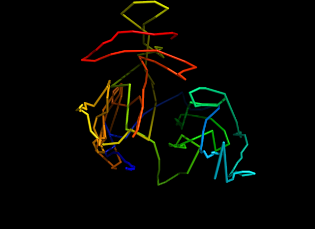
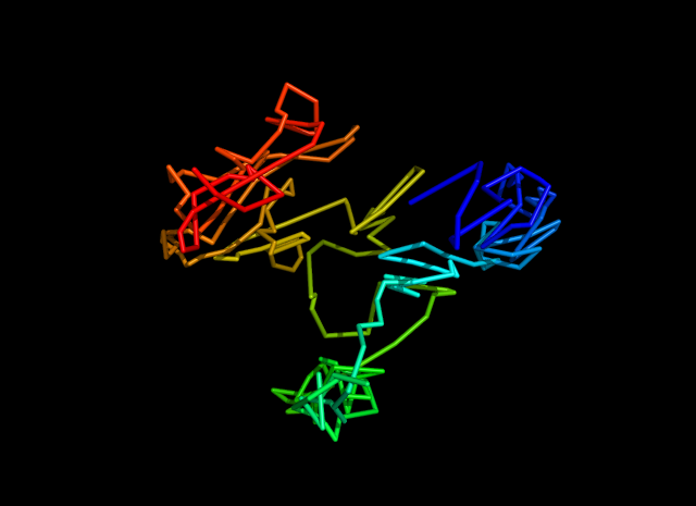
We found PYMOL is a good tool to visualize the 3D structure.

Here is the code to generate a movie for 3D structure rotating 360.

mset 1, 180
util.mroll 1, 180, 1
set ray_trace_frames, 1
set cache_frames, 0

Here is the estimated structure.

1. Objective function with biological constraints.

2. Robust analysis

---